23 min to read
Remote sensing Nakuru's urban growth (2) | geemap + Google Earth Engine
Data: Landsat 7-8 | Tools: geemap (Google Earth Engine), Jupyter-Notebook
This is the second in a three part series telling the story of Nakuru’s urban expansion using different technologies. While Part 1 employed proprietary software (ERDAS IMAGINE) to produce static images, Part 2 will employ the open-source geemap package and the Jupyter Notebook to source the data from the Google Earth Engine Data Catalog, conduct a supervised classification in the cloud and produce an interactive map - all without having to download a single large datasets to your harddrive.
If this is your first time working with geemap, or virtual conda environments, geemap’s tutorials will guide you through installing the package and taking your first steps. The workflow below partly follows geemap tutorial no. 32.
Downloads: You can download the accompanying Jupyter Notebook here which will allow you to avail of the interactive features.
Or directly jump to the live app here (it may take about 30 seconds to load), built using heroku.
- Getting started
- Adding a reference layer and generating sample points
- Training the classifier
- Classifying a Landsat 8 scene from 2020
- Simplifying land cover classes
- Classifying a Landsat 8 scene from 2013
- Classifying a Landsat 7 scene from 2002
- Final output
- Annex - Manual sample collection
Getting started
We first import geemap and the GEE Python API. We then define the region of interest we already used in Part 1. Finally, we instantiate a geemap Map object and center the resulting leaflet map on our region of interest to get our bearings.
import geemap
import ee
import ipywidgets as widgets
ee.Initialize()

roi = ee.Geometry.Polygon(
        [[[35.750324, -0.480940],
          [35.750324, -0.108933],
          [36.261697, -0.108933],
          [36.261697, -0.480940],
          [35.750324, -0.480940]]], None, False)

Map = geemap.Map()
Map.centerObject(roi, zoom=11)
Map
Next we add a Landsat 8 scene from around the time (2018-19) of the latest issue of the 100m resolution Copernicus CGLS-LC100 Collection 3 land cover dataset which we will use to train a classifier. While not a perfect match, this should be a sufficient approximation. We sort the ImageCollection by cloud cover, select the first of these and clip the scene to our region of interest.
Let’s also verify the scene’s percentage of cloud cover.
L8_2018 = ee.ImageCollection("LANDSAT/LC08/C01/T1") \
    .filterBounds(roi) \
    .filterDate('2018-10-01', '2018-10-31') \
    .sort('CLOUD_COVER') \
    .first() \
    .clip(roi)

L8_2018.get('CLOUD_COVER').getInfo()
2.1500000953674316
Let’s add this to our map as a true color composite, though we could just as well skip this step.
vis_params = {'min': 0,
    'max': 25000,'bands': ['B4','B3', 'B2']}

Map.addLayer(L8_2018, vis_params, "Landsat 8, raw (2018)")
Adding a reference layer and generating sample points
Next, we add the latest Copernicus land cover dataset, again clipping it to our ROI.
We should also compare the dates of acquisition for the training and input dataset to make sure they’re roughly in the same ballpark.
copernicus_lc = ee.ImageCollection("COPERNICUS/Landcover/100m/Proba-V-C3/Global") \
    .select("discrete_classification") \
    .sort('system:time_start', False) \
    .first() \
    .clip(roi)

print("Landsat 8 date of acquisition: ", ee.Date(L8_2018.get('system:time_start')).format('YYYY-MM-dd').getInfo())
print("Copernicus issue date: ", ee.Date(copernicus_lc.get('system:time_start')).format('YYYY-MM-dd').getInfo())
Landsat 8 date of acquisition:  2018-10-03
Copernicus issue date:  2019-01-01
Next, we’ll generate a FeatureCollection of 10,000 random points across our ROI and have each point sample the land cover classification data from Copernicus (as can be seen by examining the first point in the FeatureCollection below).
# generating 5,000 random points
points = copernicus_lc.sample(**{
    'region': roi,
    'scale': 30,
    'numPixels': 10000,
    'seed': 0,
    'geometries': True  # Set this to False to ignore geometries
})

print(points.first().getInfo())
{'type': 'Feature', 'geometry': {'type': 'Point', 'coordinates': [35.9493404834219, -0.42350413564375233]}, 'id': '0', 'properties': {'discrete_classification': 40}}
Training the classifier
In this step, each band’s pixel values from Landsat 8 will be added to the attributes of the points FeatureCollection which we’ll then use to train the classifier.
# Use these bands of the Landsat 8 scene for predicting the likely land cover class
bands = ['B1', 'B2', 'B3', 'B4', 'B5', 'B6', 'B7', 'B10', 'B11']


# This band in the Copernicus ImageCollection stores the actual numeric land cover information
# which we will use for training the classifier
# see: https://developers.google.com/earth-engine/datasets/catalog/COPERNICUS_Landcover_100m_Proba-V-C3_Global#bands
label = 'discrete_classification'

# Overlay the points on the imagery to get training.
# see: https://developers.google.com/earth-engine/apidocs/ee-image-sampleregions
training = L8_2018.select(bands).sampleRegions(**{
  'collection': points,
  'properties': [label],
  'scale': 30
})

# Here we choose the Random Forest algorithm with 15 decision trees.
# Feel free to experiment with either this number or any of the other algorithms available.
# Some, like Support Vector Machines, will take significantly longer to complete.
# see here and following: https://developers.google.com/earth-engine/apidocs/ee-classifier-amnhmaxent
classifier = ee.Classifier.smileRandomForest(15).train(training, label, bands)
print(training.first().getInfo())
{'type': 'Feature', 'geometry': None, 'id': '0_0', 'properties': {'B1': 9366, 'B10': 28289, 'B11': 25491, 'B2': 8740, 'B3': 8993, 'B4': 8354, 'B5': 18700, 'B6': 14156, 'B7': 10355, 'discrete_classification': 40}}
Classifying a Landsat 8 scene from 2020
This is where the rubber hits the road and we actually classify a Landsat 8 scene based on the Copernicus training data we just collected. The scene we’re going to classify, however, will not be the one we used for training but instead the same scene we manually classified in Part 1.
L8_2020 = ee.ImageCollection("LANDSAT/LC08/C01/T1") \
    .filterBounds(roi) \
    .filterDate('2020-10-08', '2020-10-09') \
    .sort('system:time_start') \
    .first() \
    .clip(roi)

# Classify the image using the same bands used for training.
result_2020 = L8_2020.select(bands).classify(classifier)

# Display the classified image with random colors.
Map.addLayer(result_2020.randomVisualizer(), {}, 'Landcover (random colors)')
Map
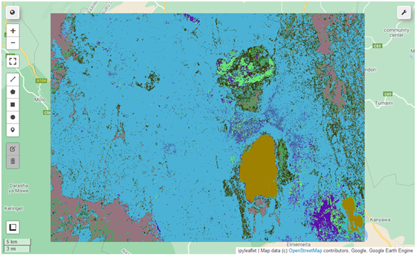
Simplifying land cover classes
Our brains have difficulty differentiating more than 10 or 12 colors at a time, let alone 23 as in this case. That’s why it will make sense to merge many of the classes into one. In our case, four main classes may be enough to tell a compelling story.
But first, we need to understand which of the numeric values correspond to which real-world land cover classes. For this, we could either simply check the discrete_classification Class Table on this page, or extract the class names and values form the dataset itself, and ‘zip’ these two lists into one.
class_values = copernicus_lc.get('discrete_classification_class_values').getInfo()
class_names = copernicus_lc.get('discrete_classification_class_names').getInfo()

zipped = list(zip(class_values, class_names))
zipped
[(0, 'Unknown. No or not enough satellite data available.'),
 (20,
  'Shrubs. Woody perennial plants with persistent and woody stems and without any defined main stem being less than 5 m tall. The shrub foliage can be either evergreen or deciduous.'),
 (30,
  'Herbaceous vegetation. Plants without persistent stem or shoots above ground and lacking definite firm structure. Tree and shrub cover is less than 10 %.'),
 (40,
  'Cultivated and managed vegetation / agriculture. Lands covered with temporary crops followed by harvest and a bare soil period (e.g., single and multiple cropping systems). Note that perennial woody crops will be classified as the appropriate forest or shrub land cover type.'),
 (50,
  'Urban / built up. Land covered by buildings and other man-made structures.'),
 (60,
  'Bare / sparse vegetation. Lands with exposed soil, sand, or rocks and never has more than 10 % vegetated cover during any time of the year.'),
 (70, 'Snow and ice. Lands under snow or ice cover throughout the year.'),
 (80,
  'Permanent water bodies. Lakes, reservoirs, and rivers. Can be either fresh or salt-water bodies.'),
 (90,
  'Herbaceous wetland. Lands with a permanent mixture of water and herbaceous or woody vegetation. The vegetation can be present in either salt, brackish, or fresh water.'),
 (100, 'Moss and lichen.'),
 (111,
  'Closed forest, evergreen needle leaf. Tree canopy >70 %, almost all needle leaf trees remain green all year. Canopy is never without green foliage.'),
 (112,
  'Closed forest, evergreen broad leaf. Tree canopy >70 %, almost all broadleaf trees remain green year round. Canopy is never without green foliage.'),
 (113,
  'Closed forest, deciduous needle leaf. Tree canopy >70 %, consists of seasonal needle leaf tree communities with an annual cycle of leaf-on and leaf-off periods.'),
 (114,
  'Closed forest, deciduous broad leaf. Tree canopy >70 %, consists of seasonal broadleaf tree communities with an annual cycle of leaf-on and leaf-off periods.'),
 (115, 'Closed forest, mixed.'),
 (116, 'Closed forest, not matching any of the other definitions.'),
 (121,
  'Open forest, evergreen needle leaf. Top layer- trees 15-70 % and second layer- mixed of shrubs and grassland, almost all needle leaf trees remain green all year. Canopy is never without green foliage.'),
 (122,
  'Open forest, evergreen broad leaf. Top layer- trees 15-70 % and second layer- mixed of shrubs and grassland, almost all broadleaf trees remain green year round. Canopy is never without green foliage.'),
 (123,
  'Open forest, deciduous needle leaf. Top layer- trees 15-70 % and second layer- mixed of shrubs and grassland, consists of seasonal needle leaf tree communities with an annual cycle of leaf-on and leaf-off periods.'),
 (124,
  'Open forest, deciduous broad leaf. Top layer- trees 15-70 % and second layer- mixed of shrubs and grassland, consists of seasonal broadleaf tree communities with an annual cycle of leaf-on and leaf-off periods.'),
 (125, 'Open forest, mixed.'),
 (126, 'Open forest, not matching any of the other definitions.'),
 (200, 'Oceans, seas. Can be either fresh or salt-water bodies.')]
Next, we create lists of equal length with the old and new values for each of the four landcover classes we envision, finally combining them into two ordered composite lists. These then go into the .remap() method for our image.
urban_orig = [50]
urban_new = [1]

natveg_orig = [20, 30, 90, 100, 111, 112, 113, 114, 115, 116, 121, 122, 123, 124, 125, 126]
natveg_new = [2, 2, 2, 2, 2, 2, 2, 2, 2, 2, 2, 2, 2, 2, 2, 2]

nonurb_orig = [0, 40, 60, 70, 200]
nonurb_new = [3, 3, 3, 3, 3]

water_orig = [80]
water_new = [4]

orig = urban_orig + natveg_orig + nonurb_orig + water_orig
new = urban_new + natveg_new + nonurb_new + water_new

# Remap the new consecutive integer values to the new ones
final_2020 = result_2020.remap(orig, new)
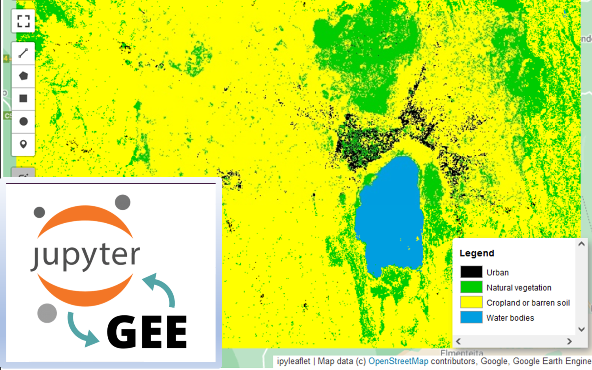
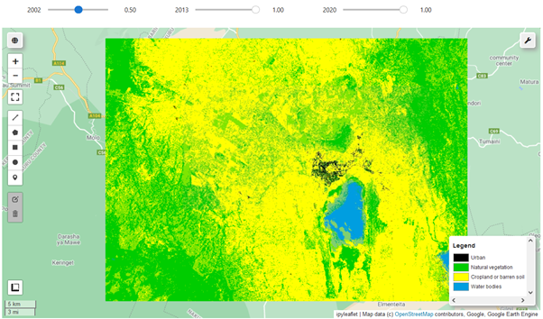
Lastly, we define legend keys and an ordered color palette which will inform both our vis_params in the addLayer method as well as the symbology for our legend.
legend_keys = ['Urban', 'Natural vegetation', 'Cropland or barren soil', 'Water bodies']

class_palette = ['000000', '00CC00', 'FFFF00', '009EE0']

Map.add_legend(legend_keys=legend_keys, legend_colors=class_palette, position='bottomright')

Map.addLayer(final_2020, {'palette': class_palette}, 'Landcover (2020)')

# remove the layers we don't need
Map.remove_layer(Map.find_layer('Landsat 8, raw (2018)'))
Map.remove_layer(Map.find_layer('Landcover (random colors)'))

Map
Classifying a Landsat 8 scene from 2013
Let’s now also classify a Landsat 8 scene from right after the satellite’s launch in 2013 but still in the month of October, just like the 2020 one.
# This gives us a scene from 5 October, 2013
L8_2013 = ee.ImageCollection("LANDSAT/LC08/C01/T1") \
    .filterBounds(roi) \
    .filterDate('2013-10-01', '2013-10-31') \
    .sort('CLOUD_COVER') \
    .first() \
    .clip(roi)

# Classify the image using the same bands used for training.
result_2013 = L8_2013.select(bands).classify(classifier)

final_2013 = result_2013.remap(orig, new)

Map.addLayer(final_2013, {'palette': class_palette}, 'Landcover (2013)')
Classifying a Landsat 7 scene from 2002
As our analysis in Part 1 began in 2002, let’s also classify the same scene here using Google Earth Engine. This time, though, we’ll use the MCD12Q1.006 MODIS Land Cover Type Yearly Global 500m as our training dataset since this started providing data in 2001. Specifically, we’ll use the University of Maryland classification (band name ‘LC_Type2’).
With a 500m ground resolution, this dataset is a lot coarser, so the results will not be as accurate as with the 100m Copernicus dataset.
L7_2002 = ee.ImageCollection('LANDSAT/LE07/C01/T1') \
    .filterBounds(roi) \
    .filterDate('2002-09-13', '2002-09-14') \
    .sort('system:time_start') \
    .first() \
    .clip(roi)

MCD_500 = ee.ImageCollection("MODIS/006/MCD12Q1") \
    .select("LC_Type2") \
    .filterDate('2003-01-01') \
    .first()

# generating 5,000 random points
points2 = MCD_500.sample(**{
    'region': roi,
    'scale': 30,
    'numPixels': 10000,
    'seed': 0,
    'geometries': True  # Set this to False to ignore geometries
})
# Slight adjustments to the bands since L7's are different to L8's
bands2 = ['B1', 'B2', 'B3', 'B4', 'B5', 'B7']

# Adjust label name
label2 = 'LC_Type2'

training2 = L7_2002.select(bands2).sampleRegions(**{
  'collection': points2,
  'properties': [label2],
  'scale': 30
})

classifier2 = ee.Classifier.smileRandomForest(15).train(training2, label2, bands2)

result_2002 = L7_2002.select(bands2).classify(classifier2)
As before, we’ll recode the landcover types into four very broad categories. Feel free to follow a more finegrained approach here.
urban_orig = [13]
urban_new = [1]

natveg_orig = [1, 2, 3, 4, 5, 6, 7, 8, 9]
natveg_new = [2, 2, 2, 2, 2, 2, 2, 2, 2]

nonurb_orig = [10, 12, 14, 15]
nonurb_new = [3, 3, 3, 3]

water_orig = [0, 11]
water_new = [4, 4]

orig = urban_orig + natveg_orig + nonurb_orig + water_orig
new = urban_new + natveg_new + nonurb_new + water_new

# Remap the new consecutive integer values to the new ones and add the new layer
final_2002 = result_2002.remap(orig, new).clip(roi)

Map.addLayer(final_2002, {'palette': class_palette}, 'Landcover (2002)')

# finally, we can add some sliders to more directly control the opacity

lc_2002 = Map.layers[-1]
lc_2013 = Map.layers[-2]
lc_2020 = Map.layers[-3]

opacity_2002 = widgets.FloatSlider(min=0, max=1, step=0.1, value=1, description="2002")
opacity_2013 = widgets.FloatSlider(min=0, max=1, step=0.1, value=1, description="2013")
opacity_2020 = widgets.FloatSlider(min=0, max=1, step=0.1, value=1, description="2020")

lc_2002.interact(opacity=opacity_2002)
lc_2013.interact(opacity=opacity_2013)
lc_2020.interact(opacity=opacity_2020)

hbox = widgets.HBox([opacity_2002, opacity_2013, opacity_2020])
hbox
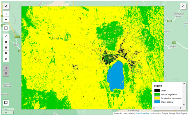
Final output
And this is the final result. You can tick and untick the three layers and adjust the layer opacity via the slider widgets above the map or in the layer control in the top right. Due to the two satellites and training datasets involved, the results are not 100% comparable, but close enough. You will also see significant differences in classification between the results here and those in Part 1. There are plenty of moving parts and, if your are so inclined, you are free to experiment both with other training datasets and classifiers at your disposal, each with their own set of parameters. In any case, the main purpose here was to introduce the significant capabilities of both geemap, Google Earth Engine and the Python environment for scalable remote sensing applications.
As always, critique and comments are more than welcome.
Annex - Manual sample collection
But what do you do if you don’t have a very good (or any) training dataset or simply want to collect samples yourself based on your own experience? The workflow below is an attempt at doing just that, though the low number of classes used will give your very mixed results. If you have the time, I recommend first sampling at least 6-8 classes and merging those after.
We will have to collect at least 20 sample points for each information class we plan to classify. Every time we’re done sampling, we need to assign the drawn features to a FeatureCollection and define a property for each feature. This then tells the classifier which landcover class we think this pixel represents. It helps to inspect the spectral profile of each area or pixel via the “Plotting” tool in the control panel prior to placing a marker, to confirm that the spectral profile matches with the type of landcover we’re currently collecting samples for. Adjusting the vis_params to other band combinations (e.g. 4-3-2 for vegetation or 4-5-3 for urban) may also help to visually hone in on certain areas.
So let’s get to it.
# First, place at least 20 markers onto urban areas using any map instance created.

# Once you're done collecting, assign those markers to a FeatureCollection

urban = ee.FeatureCollection(Map.draw_features)

# then, define a function which will set a 'class' property to the value of a global scope variable
# we set prior to calling the map function

def set_class(feature):
    return feature.set({'class': class_val})

class_val = 1

urban = urban.map(set_class)

# Let's verify that this worked
print(urban.first().getInfo())
Now clear the drawn features via the respective button in the control panel in the top right of the map.
We’ll now collect samples for natural vegetation. Set the vis_params to a NIR false color composite (4-3-2) and pick out pixels in deep red. When you’re done collecting, again assign the drawn features to a FeatureCollection and set their ‘class’ property
natveg = ee.FeatureCollection(Map.draw_features)

class_val = 2

natveg = natveg.map(set_class)

print(natveg.first().getInfo())
# By now, you know the drill: clear, collect, assign and set_class

nonurb = ee.FeatureCollection(Map.draw_features)

class_val = 3

nonurb = nonurb.map(set_class)
# Finally, our last information class: water.

water = ee.FeatureCollection(Map.draw_features)

class_val = 4

water = water.map(set_class)
# Now, we'll merge all four FeatureCollections into one

points2 = urban.merge(natveg).merge(nonurb).merge(water)

# Let's see how many samples we have in total - clearly less than then 10,000 above, so the results are likely not going to be on par
points2.size().getInfo()
Everything from here on out is replicating what we did above.
# Slight adjustments to the bands since L7's are different to L8's, as well as the label we chose above
bands2 = ['B1', 'B2', 'B3', 'B4', 'B5', 'B7']

label2 = 'class'

training2 = L7_2002.select(bands2).sampleRegions(**{
  'collection': points2,
  'properties': [label2],
  'scale': 30
})

classifier2 = ee.Classifier.smileRandomForest(15).train(training2, label2, bands2)
final_2002 = L7_2002.select(bands2).classify(classifier2)

# final_2002 = result_2002.remap(orig, new)

Map.addLayer(final_2002, {'min': 1, 'max': 4, 'palette': class_palette}, 'Landcover (2002)')

Map

Comments