9 min to read
OSM, but your way | GeoViews, datashader, Bokeh Server
Data: OpenStreetMap | Tools: osmnx, GeoViews, datashader, Bokeh Server
Want to quickly source building footprints, road geometries, or points of interest in places where vector data is hard to come by? Want to visualise your, potentially, millions of features interactively in the browser with the performance of a tile layer while having the freedom to customise symbology and inspect features as if working directly with vector data? If any of this sounds intriguing to you, do read on.
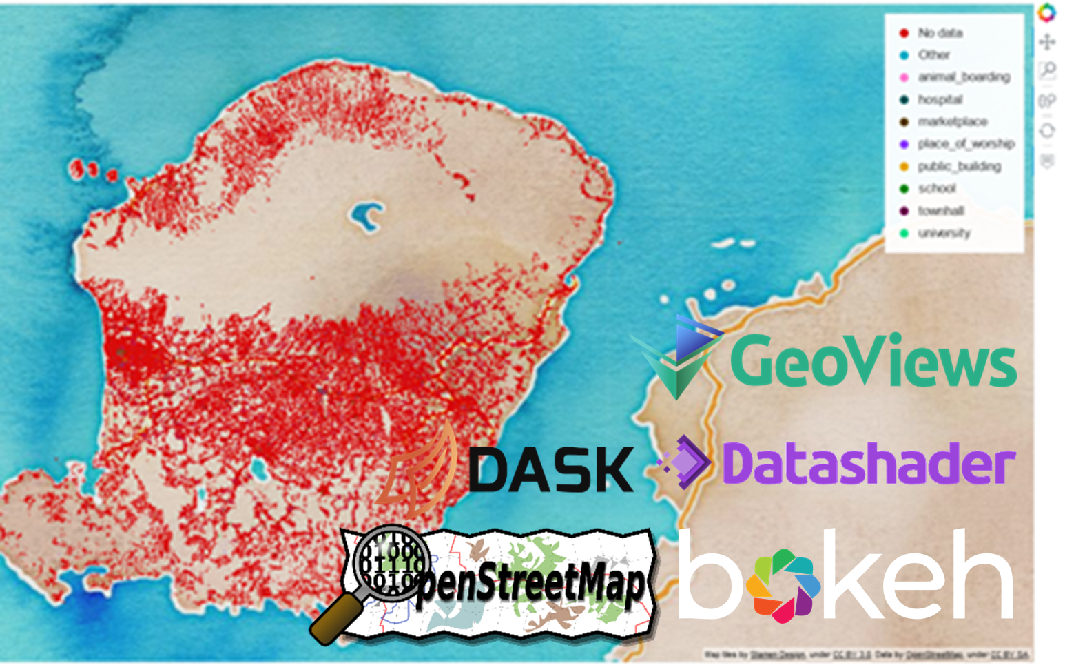
In this short post, we will source building footprints for a user-defined region of interest (ROI), in this case the island of Lombok, from OpenStreetMap using osmnx and save them efficiently to disk using Dask/fastparquet. We will then use GeoViews and datashader, two libraries in the incredible suit of tools maintained by HoloViz, to dynamically turn only those polygons visible in the browser's viewport into raster representations with a custom symbology based on a categorical feature attribute. We then send this data to a live instance of Bokeh Server on localhost. You can download the accompanying Python module here.
In the next installment, we'll look at deploying our app on a GCP Linux instance.
Defining the ROI
If you know your ROI coordinates in WGS84 already, you can skip this step and simply define your polygon manually. If not, we can quickly do this in QGIS by, for instance, adding an OSM tile layer to an empty map, zooming in on our area of interest, creating a polygon layer in a GeoPackage ( Browser panel, Create Database ) in the same location as our Python module and adding a polygon feature to the layer representing our ROI ( Toggle Editing in the layer's context menu and Add Polygon Feature button).
Environment and imports
You can download an environment.yml here and recreate the major dependencies of the environment used for this demo.
Below are the imports and some optional external resources required for our application.
# app.py

import os
import osmnx as ox
import geopandas as gpd
import spatialpandas
import spatialpandas.io
from cartopy import crs as ccrs
import geoviews as gv
import datashader as ds
from holoviews.operation.datashader import (
    datashade, inspect_polygons
)
from bokeh.models import HoverTool
from colormap import rgb2hex
import colorcet as cc

gv.extension('bokeh')

# Manual inputs
gpkg_path = 'data.gpkg'
roi_layer = 'study_area'
parq_path = 'buildings.parq'
Preparing the script
To be considerate of OSM being a free service, when we run the script for the first time we’ll write whatever we retrieve to file using fastparquet, to then be retrieved in case the script is re-executed, e.g. when the cloud instance restarts or we simply changed something.
if os.path.exists(parq_path):

    spd_gdf = spatialpandas.io.read_parquet(parq_path)

    cats = list(spd_gdf.amenity.value_counts().iloc[:10].index.values)

else:

    roi = gpd.read_file(gpkg_path, layer=roi_layer)

    # get all the buildings within the ROI
    gpd_gdf = ox.geometries_from_polygon(roi.geometry[0], {'building': True})

    # OSM features with building=True occasionally include point features as well
    # Let's filter those out
    gpd_gdf = gpd_gdf[gpd_gdf.geom_type == 'Polygon'].to_crs(epsg=3857)

    # We're now converting the GeoPandas GDF to a SpatialPandas GDF
    spd_gdf = spatialpandas.GeoDataFrame(gpd_gdf)
Note that OSM’s ‘nodes’ column is a list. Apart from causing trouble when saving to GPKG or SHP, leaving the datatype as is also throws a non-obvious value error when using datashader (ValueError: The truth value of an array with more than one element is ambiguous. Use a.any() or a.all()). Therefore we’re converting the nodes column to a string, removing the square brackets at either end.
When we’re done prepping the dataframe, we’ll write to file using fastparquet.
    spd_gdf['nodes'] = str(spd_gdf['nodes'])[1:-1]

    # The default no data value for OSM is 'NaN'
    # Let's rename this to make it more obvious to new user
    spd_gdf['amenity'] = spd_gdf.amenity.fillna('No data')
    spd_gdf['name'] = spd_gdf.name.fillna('No data')
    spd_gdf['description'] = spd_gdf.description.fillna('No data')

    # Here we select the 9 most frequent amentiy categories in the dataset,
    # define all others as 'Other' and create a new category list
    # including 'Other'
    cats = list(spd_gdf.amenity.value_counts().iloc[:9].index.values)
    spd_gdf['amenity'].loc[~spd_gdf['amenity'].isin(cats)] = 'Other'
    cats = list(spd_gdf.amenity.value_counts().iloc[:10].index.values)

    # as we'll be applying datashader to the 'amenity' column we'll have to give it the 'category' type
    spd_gdf['amenity'] = spd_gdf['amenity'].astype('category')

    # then we save the dataframe to a parquet file for future use
    spd_gdf.to_parquet(parq_path)
Next we’ll prepare the legend and what we want our interactive map to look like. We first select a categorical color map suitable for lighter backgrounds, here with a maximum lightness (“maxl”) of 70 (further info here).
We also create a dict where each category key is assigned a value composed of a three element tuple of integers representing a color in RGB format. (This I then had to convert to hex as Bokeh was throwing errors otherwise.)
colors = cc.glasbey_bw_minc_20_maxl_70

color_key = {cat: rgb2hex(*tuple(int(e*255.) for e in colors[i])) for i, cat in enumerate(cats)}

# This is a temporary legend workaround
legend = gv.NdOverlay({k: gv.Points([0,0], label=str(k)).opts(
                                        color=v, apply_ranges=False)
                        for k, v in color_key.items()}, 'amenity')
Finally, Bokeh is used to define the hover tool, GeoViews to handle geometries and our tile basemap provided by Stamen, and datashader to transform/rasterise polygons based on their ‘amenity’ attribute, utilising the same color key we defined above.
polys = gv.Polygons(spd_gdf, crs=ccrs.GOOGLE_MERCATOR, vdims='amenity')

# the content of these columns will be displayed via the hover tool
tooltips = [('Amenity type', '@amenity'),
            ('Description', '@description'),
            ('Name','@name')]

hover_tool = HoverTool(tooltips=tooltips)

shaded = datashade(polys, color_key=color_key, aggregator=ds.by('amenity', ds.any()))
hover = inspect_polygons(shaded).opts(fill_color='yellow', tools=[hover_tool])

tiles = gv.tile_sources.StamenWatercolor().opts(xaxis=None, yaxis=None,active_tools=['wheel_zoom'], min_height=700, responsive=True)

overlay = tiles * shaded * hover * legend
Since we now have an overlay composed of all the individual elements, we can define a server document for Bokeh Server to use and give our app a name to display in the browser tab.
doc = gv.renderer('bokeh').server_doc(overlay)
doc.title = 'GeoViews + Datashader + Bokeh App'
Launching Bokeh Server
To launch the Bokeh Server, activate your conda environment, change to your module’s directory and run
bokeh serve app.py –-show
Depending on the size of your ROI, the session token may expire before osmnx has finished downloading. To increase the token duration beyond the default of (I believe) 15 minutes, add the –session-token-expiration command followed by the expiration duration in milliseconds, e.g.
bokeh serve app.py –-show --session-token-expiration 1200000
Do note that it’s often easier to test on smaller ROIs before scaling up to larger ones.
Final output
The demo below covers all 1,240,867 building footprints recorded on OSM for Lombok island as of 17 October 2021, color-coded by building use. As you can see, when zooming in, the raster representations of the polygons will briefly become quite obvious before datashader generates new raster representations for the current zoom level. When hovering over individual buildings, the polygon's attributes we specified will be displayed interactively.
Neat, no? :)

Comments